How to Optimize AI Models for Production
Practical techniques for improving model performance, reducing latency, and lowering costs.
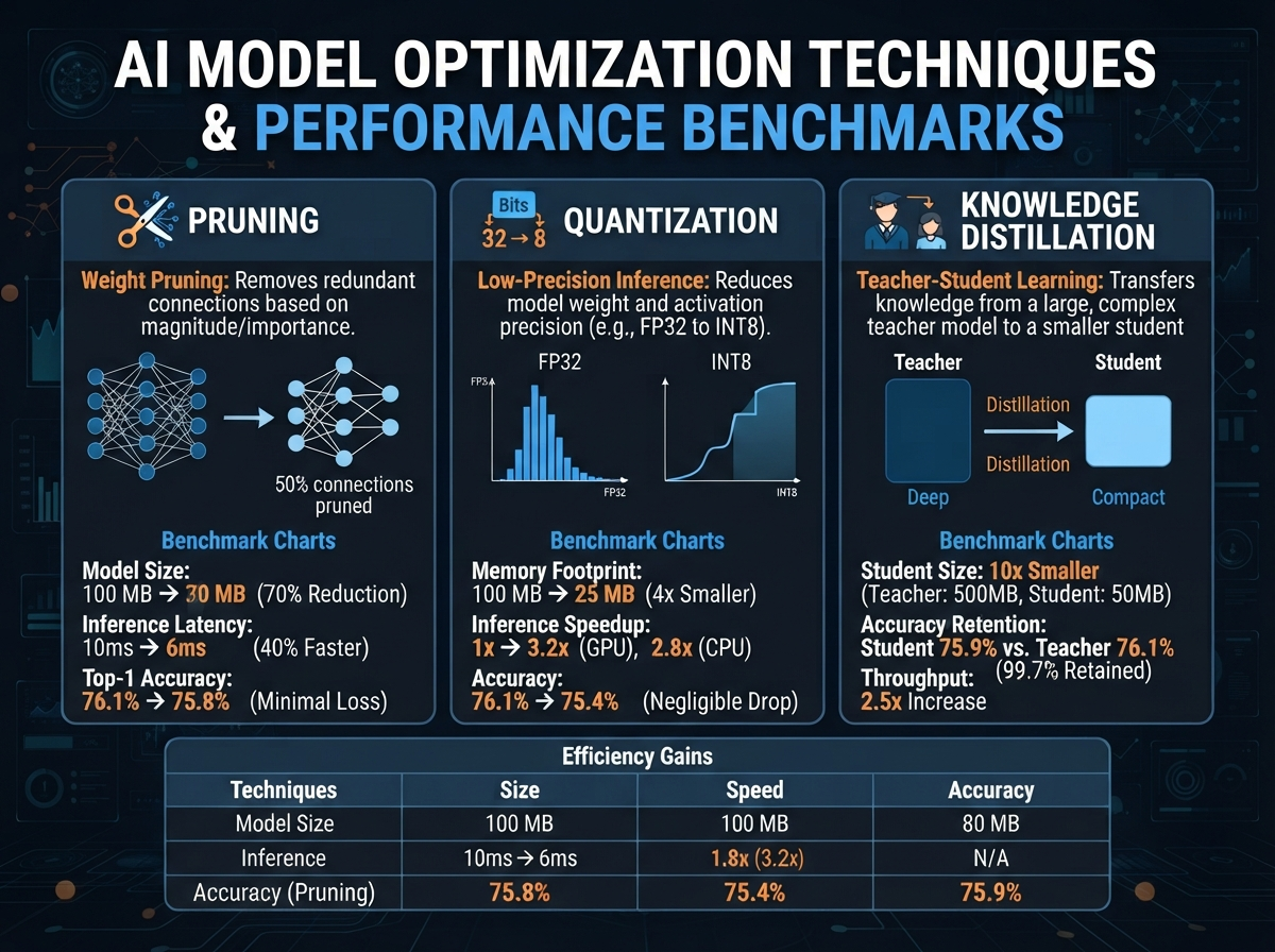
Model optimization reduces costs, improves latency, and maintains quality. This guide covers the most effective optimization techniques.
Step 1: Measure Current Performance
Establish baselines before optimizing:
import time

def benchmark_model(model, test_data):
    start_time = time.time()
    predictions = model.predict(test_data)
    latency = (time.time() - start_time) / len(test_data) * 1000  # ms

    accuracy = evaluate_accuracy(predictions, test_data.labels)

    return {
        'latency_ms': latency,
        'accuracy': accuracy,
        'throughput': len(test_data) / latency * 1000
    }

baseline = benchmark_model(model, test_data)
print(f"Baseline - Latency: {baseline['latency_ms']:.2f}ms, Accuracy: {baseline['accuracy']:.2%}")
Step 2: Quantization
Reduce model size and improve speed:
Post-Training Quantization
from transformers import AutoModelForSequenceClassification
import torch

# Load model
model = AutoModelForSequenceClassification.from_pretrained("bert-base")

# Quantize to int8
model.to('cpu')
quantized_model = torch.quantization.quantize_dynamic(
    model,
    {torch.nn.Linear},
    dtype=torch.qint8
)

# Check size reduction
original_size = sum(p.numel() * 4 for p in model.parameters()) / 1e6  # MB
quantized_size = sum(p.numel() * 1 for p in quantized_model.parameters()) / 1e6
print(f"Size reduction: {original_size:.0f}MB → {quantized_size:.0f}MB ({quantized_size/original_size*100:.0f}%)")
Quantization Results
- Model size: 75-90% reduction
- Latency: 2-4x speedup
- Accuracy loss: 0-2% (usually minimal)
Step 3: Model Compression
Pruning
import torch.nn.utils.prune as prune

# Prune 30% of weights
for module in model.modules():
    if isinstance(module, torch.nn.Linear):
        prune.l1_unstructured(module, name='weight', amount=0.3)
        prune.remove(module, 'weight')

# Check sparsity
total_params = sum(p.numel() for p in model.parameters())
zero_params = sum((p == 0).sum() for p in model.parameters())
sparsity = zero_params / total_params
print(f"Model sparsity: {sparsity:.1%}")
Knowledge Distillation
class DistilledModel(torch.nn.Module):
    def __init__(self, teacher_model):
        super().__init__()
        # Create smaller model
        self.student = create_small_model()
        self.teacher = teacher_model
        self.temperature = 4.0

    def forward(self, x):
        student_output = self.student(x)
        teacher_output = self.teacher(x)

        # Use teacher to guide student
        loss = self.distillation_loss(
            student_output,
            teacher_output,
            self.temperature
        )
        return loss
Step 4: Caching and Batching
Caching Results
from functools import lru_cache

@lru_cache(maxsize=10000)
def get_prediction(input_hash):
    # Return cached result if available
    return model.predict(input_hash)
Request Batching
import asyncio

class BatchPredictor:
    def __init__(self, batch_size=32):
        self.batch_size = batch_size
        self.batch = []

    async def predict(self, input_data):
        self.batch.append(input_data)
        if len(self.batch) >= self.batch_size:
            return await self.process_batch()

    async def process_batch(self):
        predictions = model.predict_batch(self.batch)
        self.batch = []
        return predictions
Step 5: Hardware Acceleration
GPU Utilization
# Move model to GPU
device = torch.device('cuda' if torch.cuda.is_available() else 'cpu')
model.to(device)

# Use half precision (FP16)
model.half()

# Optimize computation
with torch.cuda.amp.autocast():
    output = model(input_data)
Specialized Hardware
- NVIDIA TensorRT: 10-100x speedup for specific hardware
- ONNX Runtime: Cross-platform optimization
- TPUs: Google’s specialized hardware
- Edge Devices: Run models on-device
Step 6: Model Architecture Optimization
Simplify Architecture
# Before: Large model
original = BERT(vocab_size=30522, hidden_size=768, num_layers=12)

# After: Smaller, faster model
optimized = BERT(vocab_size=30522, hidden_size=384, num_layers=6)

# Trade-offs:
# - 75% fewer parameters
# - 3x faster inference
# - 1-2% accuracy drop
Step 7: Profiling
Identify bottlenecks:
import cProfile
import pstats

profiler = cProfile.Profile()
profiler.enable()

# Run model
predictions = model.predict(test_data)

profiler.disable()
stats = pstats.Stats(profiler)
stats.sort_stats('cumulative')
stats.print_stats(10)  # Print top 10
Optimization Techniques Comparison
| Technique | Latency Improvement | Memory Reduction | Accuracy Impact |
|---|---|---|---|
| Quantization | 2-4x | 75% | 0-2% |
| Pruning | 1.5-2x | 30-50% | 1-3% |
| Distillation | 2-3x | 90% | 2-5% |
| Compilation | 1.5-2x | 0% | 0% |
Optimization Strategy
- Measure: Establish baseline metrics
- Profile: Find bottlenecks
- Optimize: Apply techniques systematically
- Test: Verify accuracy maintained
- Deploy: Monitor production performance
Real-World Example
Original BERT Model:
- Latency: 150ms
- Model size: 400MB
- Accuracy: 92%
After Optimization:
- Latency: 30ms (5x faster)
- Model size: 80MB (80% smaller)
- Accuracy: 90% (2% loss)
Conclusion
Smart optimization can dramatically improve performance while maintaining model quality. Start with profiling to identify bottlenecks, then apply techniques systematically.
Sources & Resources
Framework Optimization
- PyTorch Quantization - https://pytorch.org/docs/stable/quantization.html
- TensorFlow Lite - https://www.tensorflow.org/lite
- ONNX Runtime - https://onnxruntime.ai/
Optimization Tools
- TVM - https://tvm.apache.org/
- OpenVINO - https://www.intel.com/content/www/us/en/developer/tools/openvino-toolkit/overview.html
- Hugging Face Optimum - https://huggingface.co/docs/optimum/
MLOps & Deployment
- MLflow - https://mlflow.org/
- Kubeflow - https://www.kubeflow.org/
- KServe - https://kserve.github.io/
- Hugging Face Model Optimization Toolkit
- Conference Papers on Model Compression and Quantization
Related Articles

How to Implement AI System Monitoring and Alerts
Step-by-step guide to setting up comprehensive monitoring for AI systems in production.
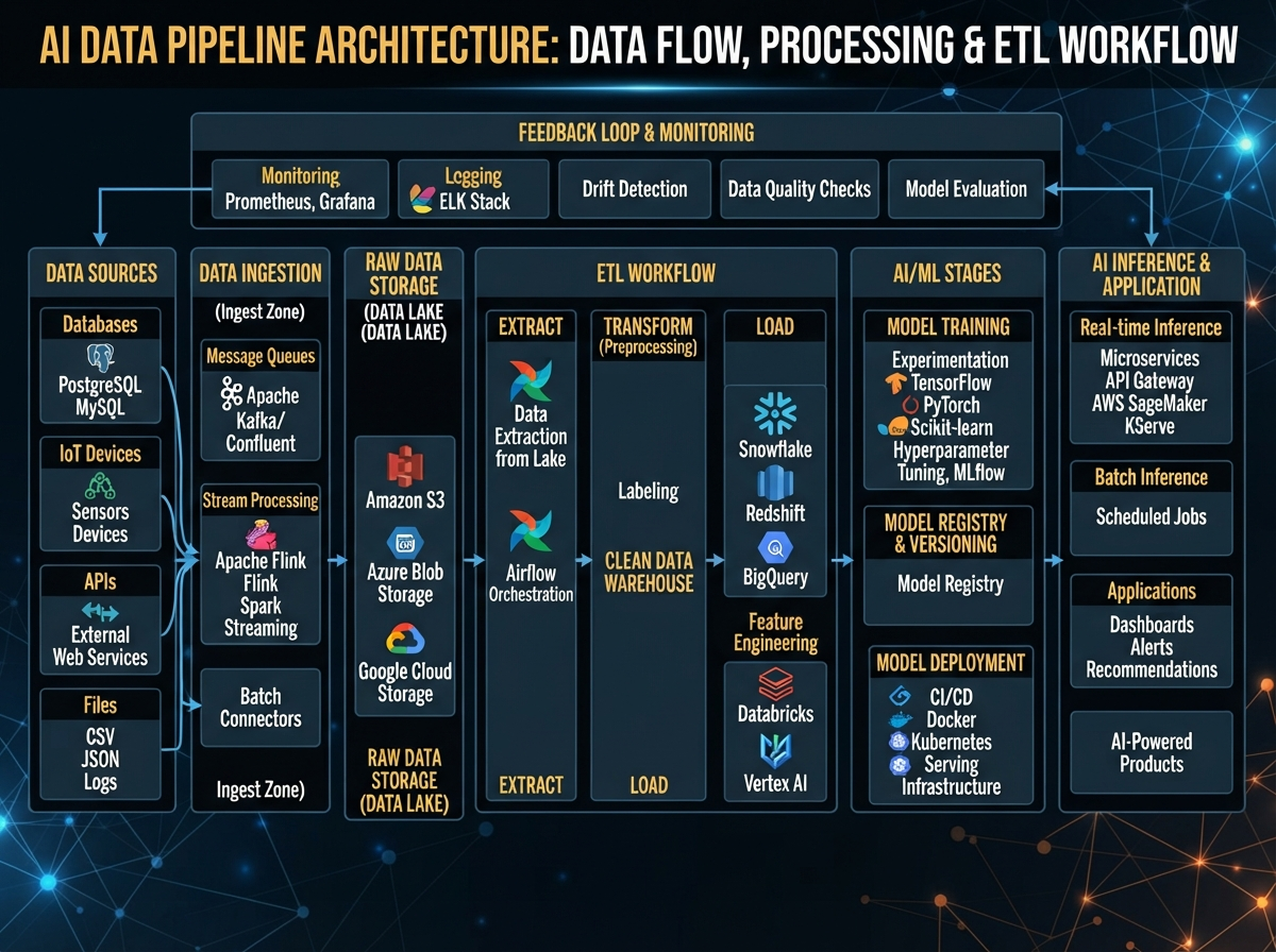
How to Build Scalable AI Data Pipelines
Step-by-step guide to building production-ready data pipelines for machine learning.
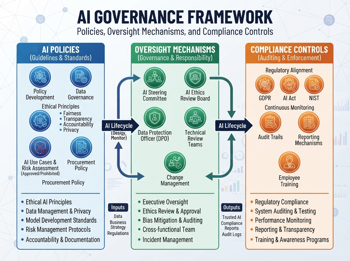
How to Implement AI Governance Frameworks
Comprehensive guide to establishing governance policies and oversight for AI systems.